MPyC demos
This is an overview of the demos available from the MPyC repository on GitHub in mpyc/demos. Starting with a ‘Hello world!’ demo, we gradually work towards demos about privacy-preserving machine learning, MPC-based threshold cryptography, and other interesting topics. Many of the more advanced demos are in fact based on research published at various cryptography conferences.
We give usage examples and also provide some high-level explanations. The Python code for these demos contains many detailed examples of how to program with MPyC.
For the more advanced demos you can use the -h switch for more detailed usage instructions.
With any demo you can also use the -H switch to consult the built-in help message for the MPyC
runtime (see MPyC command line for all options); this help message is also accessible
without any demo at hand, namely by running:
python -m mpyc -H
If you leave out -H here, you directly enter an asyncio REPL with MPyC preloaded
together with some standard secure types.
This way you can quickly experiment with all kinds of MPyC functions:
>>> await mpc.output(list(mpc.min_max(secint(7), 8, secint(-3), 3)))
[-3, 8]
The results can be viewed immediately through top-level await expressions, which you may know
already from Jupyter notebooks.
helloworld.py
Let’s start with a simple run of the ‘Hello world!’ demo:
$ python helloworld.py
2021-06-16 09:21:07,574 Start MPyC runtime v0.7.7
Hello world!
2021-06-16 09:21:07,574 Stop MPyC runtime -- elapsed time: 0:00:00
By default, an MPyC program is run with just one party, which is convenient for testing purposes. Here, the one and lonely party says hello to itself.
To test an MPyC program with multiple parties use the -M switch to set the number of parties:
$ python helloworld.py -M 5
2021-06-16 09:30:49,713 Start MPyC runtime v0.7.7
2021-06-16 09:30:50,244 All 5 parties connected.
Hello world!Hello world!Hello world!Hello world!Hello world!
2021-06-16 09:30:50,260 Stop MPyC runtime -- elapsed time: 0:00:00.546839
This causes the demo to be run with \(m=5\) parties, using a local TCP/IP connection between each pair of parties, for a total of \({m \choose 2}=10\) connections. This way, the number of connections can go to quite extreme levels, e.g., for \(m=300\) there will be a whopping 44,850 connections created on your local machine:
python helloworld.py -M300 --no-prss
provided you’ve granted your OS enough resources to handle this kind of load.
To engage in a protocol with someone else on a remote machine you can run:
python helloworld.py -P localhost -P 192.168.1.22 -I0
and your peer would run:
python helloworld.py -P 192.168.1.11 -P localhost -I1
The -P switches are used to set the IPv4 addresses for the two parties, where the order is significant and must be consistent.
To run the demo with more parties just keep adding -P switches. The port numbers will be set automatically, but can
also be specified in several ways.
The -I switch is used to assign a unique index \(i\in\{0,1,\ldots,m-1\}\) to each of the \(m\) parties.
The party’s index \(i\) is much like the rank assigned to a process(or) in a parallel computing context,
and it can be obtained as mpc.pid within a running MPyC program.
The actual code of the ‘Hello world!’ demo is very simple:
from mpyc.runtime import mpc


async def main():
    await mpc.start()
    print(''.join(await mpc.transfer('Hello world!')))
    await mpc.shutdown()

if __name__ == '__main__':
    mpc.run(main())
There is not much secrecy in this program, as the hello messages are broadcast using mpc.transfer() such that
each party gets a hello message from all other parties (including one from itself).
However, mpc.transfer() is much more powerful than this, allowing parties to send private messages between each other,
basically by specifying a (directed) communication graph which can be set arbitrarily. Also, mpc.transfer() allows the parties
to send arbitrary Python objects as messages, as long as these objects can be serialized using Python’s pickle module,
cf. what-can-be-pickled-and-unpickled.
See helloworld.py for more information.
oneliners.py
This demo presents four oneliners in MPyC, which do some actual secure computation. We run it with \(m=7\) parties, this time suppressing the log messages:
$ python oneliners.py -M7 --no-log
m    = 7
m**2 = 49
2**m = 128
m!   = 5040
We are computing some simple functions of \(m\) here, hence there is no secrecy in this respect.
The actual computations, however, are all done on secret-shared values. Let’s break down the
oneliner producing m**2 = 49 as output:
await mpc.output(mpc.sum(mpc.input(mpc.SecInt(2*l+1)(2*i+1))))
To understand the mechanics of this oneliner, we look at all intermediate results:
secint = mpc.SecInt(2*l+1)  # secure integers of bit length 2l+1
a = secint(2*i+1)           # set a = 2i+1 for party i = mpc.pid
s = mpc.input(a)            # secret-share a with all other parties
b = mpc.sum(s)              # sum of secret-shared entries of s
f = mpc.output(b)           # value of secret-shared sum in the clear
We start off with secint created dynamically as a type of “secure integers” of bit length \(2l+1\),
where \(l\) is the bit length of \(m\).
We could have used the simpler call mpc.SecInt() here, which defaults to 32-bit secure integers.
But for better performance we limit the bit length to \(2l+1\), which is chosen to be just large enough to hold
the values that we are about to compute.
Next we let party \(i\) create a secure integer a set to value \(2i+1\). The index \(i\) is obtained
from the MPyC runtime by inspecting the attribute mpc.pid. Even though these indices are known by all parties
taking part in this secure computation, the ensuing arithmetic for variable a will all be done by means of
cryptographic protocols operating on secret-shared integers.
The parties then secret-share their input through a call mpc.input(a) by which each party will obtain
a length-\(m\) list s of secure integers. For \(m=7\) the entries of s correspond to the
values \(1,3,5,7,9,11,13\). However, when the parties would inspect s from their running copies of the
MPyC program, they will not see these values. What they will be able to see are random values constituting
their shares of the entries of s.
The sum of all entries of s is computed securely and the result is assigned to b, which will also be a secure
integer. We use a call to mpc.sum(), although in this case we can also call the Python built-in
function sum(). The MPyC runtime handles the summation more efficiently.
Finally, we let the parties reconstruct the value of b in the clear. The call mpc.output(b) causes
the MPyC runtime to let the parties exchange their shares pertaining to the secure integer b, which results
in all parties seeing \(1+3+5+7+9+11+13=49\).
Technically, the value of f is a Python Future() instance, whose result will hold the value 49 as a
Python integer of type int once the evaluation of f is done. To obtain this value we can use await f
if we are inside a Python coroutine, and otherwise the call mpc.run(f) will make sure that f is evaluated.
The other oneliners can be broken down similarly. For instance, the oneliner responsible for output 2**m = 128
is:
await mpc.output(mpc.prod(mpc.input(mpc.SecInt(m+2)(2))))
Here, mpc.prod(s) securely computes the product of all entries of s. The MPyC runtime will organize
the computation of this product such that all required secure multiplications are done in a logarithmic number of rounds,
namely \(\lceil \log_2 m \rceil\) rounds to be precise.
Enfin, a lot of words to sketch how and why these MPyC oneliners work. The good news is that you should be fine forgetting most of these details when working with MPyC, as its API has been designed to let you program secure multiparty computations as if you are working with “ordinary” Python code.
See oneliners.py for more information.
unanimous.py
In this demo we see how parties actually use a private choice as input to a secure computation. The choice is between just two values, “yes” and “no” votes, which we encode as 1s and 0s, respectively. For unanimous agreement we only want to learn if everybody votes “yes”, which means that the product of all binary encodings is equal to 1. Presence of any “no” vote will make the product equal to 0.
The case of two parties Alice and Bob finding out if they’re romantically interested in each other is a special case
of unanimous agreement. When doing this in a privacy-preserving manner, we also refer to this as ![]() matching without embarrassments.
To have an honest majority we add a trusted helper as a third party.
The helper party will not provide any input.
matching without embarrassments.
To have an honest majority we add a trusted helper as a third party.
The helper party will not provide any input.
Here’s an example run between Alice, Bob, and a helper (parties \(i=0,1,2\)):
$ python unanimous.py -M3 -I0 1
No match: someone disagrees among 2 parties?
$ python unanimous.py -M3 -I1 0
No match: someone disagrees among 2 parties?
$ python unanimous.py -M3 -I2
Thanks for serving as oblivious matchmaker;)
Alice is interested in Bob, but Bob indicates that he’s not interested in Alice. They do so by providing a 1 and a 0 as input respectively. The helper party provides no input, and also gets no output, hence remains oblivious about the outcome of this matchmaking.
The mismatch is no surprise to Bob, clearly. The whole point about this particular secure computation is that Bob does not learn if Alice is interested in him or not. This bit of information remains hidden from Bob because of the privacy-preserving property of a secure computation. The only information that parties are allowed to learn is what they can deduce from the output that is demanded from the computation, combined with their knowledge about the inputs that they provide to the computation.
The unanimous agreement demo generalizes matchmaking between any number of parties. For parameter \(t\geq0\) the demo runs between \(m=2t+1\) parties in total, of which \(t+1\) parties cast a vote, and the remaining \(t\) parties act as trusted helpers. The main privacy-preserving property is that even a collusion of \(t\) voters cannot find out what the remaining vote is, of course, unless all colluding voters input a 1.
With voters = list(range(t+1)), where \(t=\lfloor m/2\rfloor\), the core of the program is formed by these two lines:
votes = mpc.input(secbit(vote), senders=voters)
result = await mpc.output(mpc.all(votes), receivers=voters)
Only the voters provide input and receive output, because senders and receivers are set accordingly in the
calls to mpc.input() and mpc.output(). Each voter provides a bit as private input, and all voters receive
the (same) result bit, which will be equal to 1 if and only if all votes are equal to 1.
The remaining parties \(i\) for \(i=t+1,\ldots,2t+1\) have no input and output, but are needed to perform
the secure multiplications for mpc.all(votes). We get maximal privacy in the sense that even if \(t\) voters conspire
against one remaining voter, they cannot find that voter’s vote (unless it can be deduced logically from result).
See unanimous.py for more information.
ot.py
In its most basic form oblivious transfer (OT) is a protocol that lets a sender transfer a message to a receiver, such that the message will reach the receiver with probability 50% (the message will be lost otherwise). The receiver will know whether the transfer is successful or not, but the sender will remain oblivious about what is happening. This somewhat weird functionality was introduced by Michael Rabin, who recognized the fundamental power of this primitive in cryptography.
The demo shows how 1-out-of-2 OT is accomplished easily if we rely on a trusted helper. The trusted helper takes part as a “third” party in the protocol, not seeing any of the transferred messages. As shown below, the trusted helper (party \(0\)) can take part in multiple OTs run in parallel between pairs of senders and receivers.
Here’s an example run with \(m=5\) parties:
$ python ot.py -M5 -I0
You are the trusted third party.
$ python ot.py -M5 -I1
You are sender 1 holding messages 46 and 10.
$ python ot.py -M5 -I2
You are sender 2 holding messages 28 and 17.
$ python ot.py -M5 -I3
You are receiver 1 with random choice bit 1.
You have received message 10.
$ python ot.py -M5 -I4
You are receiver 2 with random choice bit 0.
You have received message 28.
So, party \(0\) is the trusted helper, parties \(1, 2\) are senders, and parties \(3, 4\) are receivers.
In 1-out-of-2 OT, a sender holds two messages x[0], x[1] say of which the receiver will get exactly one, namely x[b] as
determined by its choice bit b.
The behavior of the MPyC program for this demo depends on (the index of) the party running the program.
Typically, this is done through conditionals in terms of mpc.pid. These conditionals are also used
in this demo program, to set the (random) values for the messages if party \(i\) is a sender (\(1\leq i\leq t\))
or to set the (random) value for the choice bit if party \(t+i\) is a receiver (\(1\leq i\leq t\)).
Together with the trusted helper there are \(m=2t+1\) parties in total, hence this demo works with an odd number
of parties.
The senders provide two numbers as private input to the protocol. In MPyC we use function mpc.input() to accomplish
this. Sender \(i\) will provide two numbers cast to a secure type secnum (for which we actually use secure integers).
All other parties also call mpc.input(), and they will put None as values, but also cast to the same secure type secnum.
To indicate that (only) sender \(i\) actually provides input, the index i of this party is passed as an
argument to mpc.input(). Similarly, receiver \(t+i\) provides its choice bit, also cast as a secnum (and all
other parties put None here as value, cast to a secnum).
The heart of the program looks as follows:
for i in range(1, t+1):
    x = mpc.input([secnum(message[i-1][0]), secnum(message[i-1][1])], i)
    b = mpc.input(secnum(choice[i-1]), t + i)
    a = await mpc.output(mpc.if_else(b, x[1], x[0]), t + i)
The final line arranges that only receiver \(t+i\) gets number a = x[b] as private output.
All other parties will get a = None here. The implementation of mpc.if_else(b, x[1], x[0])
will basically compute b*(x[1]-x[0])+x[0], assuming that b is a bit.
See ot.py for more information.
parallelsort.py
This demo is about parallel computation rather than secure computation. Using some basic ideas from parallel computing we can let \(m\) parties sort a list of \(n\) numbers in \(O(n)\) time in the comparison model—provided \(m\) is sufficiently large compared to \(n\).
The demo shows how to sort with several built-in Python types (e.g., integers), but also how to
do this with MPyC secure types (e.g., secure fixed-point numbers). In the latter case, however,
we do not require any secrecy for the numbers that we are sorting. To enforce this, the program
sets the threshold \(t=0\), which is accomplished by the assignment mpc.threshold = 0.
This gives the same effect as using switch -T 0 on the command line.
Here’s an example run with \(m=2\) parties:
$ python parallelsort.py -M2
2021-06-23 09:38:40,778 Start MPyC runtime v0.7.7
2021-06-23 09:38:41,296 All 2 parties connected.
====== Using MPyC integers <class 'mpyc.sectypes.SecInt32'>
Random inputs, one per party:  [64, 51]
Sorted outputs, one per party: [51, 64]
 * * *
====== Using Python integers
Random inputs, one per party:  [56, 28]
Sorted outputs, one per party: [28, 56]
Random inputs, 2 (sorted) per party: [98, 856, 733, 914]
Sorted outputs, 2 per party:         [98, 733, 856, 914]
 * * *
====== Using MPyC fixed-point numbers <class 'mpyc.sectypes.SecFxp32:16'>
Random inputs, one per party:  [-61.5, -15.5]
Sorted outputs, one per party: [-61.5, -15.5]
 * * *
====== Using Python floats
Random inputs, one per party:  [-73.5, -4.5]
Sorted outputs, one per party: [-73.5, -4.5]
Random inputs, 2 (sorted) per party: [91.0, 92.125, 4.0, 26.375]
Sorted outputs, 2 per party:         [4.0, 26.375, 91.0, 92.125]
 * * *
====== Using MPyC floats <class 'mpyc.sectypes.SecFlt32:24:8'>
Random inputs, one per party:  [9.922563918256522e+29, 6.38978648651677e+29]
Sorted outputs, one per party: [6.38978648651677e+29, 9.922563918256522e+29]
 * * *
2021-06-23 09:38:41,340 Stop MPyC runtime -- elapsed time: 0:00:00.561404
For the purpose of demonstration, the program uses two ways to exchange numbers between the parties.
For the ordinary Python types we use mpc.transfer(), while we use mpc.output(mpc.input()) for
the secure MPyC types. Since we set \(t=0\), a call to mpc.input() is equivalent to sending all
parties a copy of the input value. This value is then recovered at the receiving party by a call to
mpc.output(), which is also a trivial step if \(t=0\) as the share that each party holds
is a copy of the secret.
See parallelsort.py for more information.
sort.py
In contrast with the previous demo, this program actually performs secure sorting. For a secure sort of a list of numbers, not only the values of all numbers in the list should remain hidden, but also how the numbers are being moved around.
For this demo we start out by performing a secure random shuffle of a publicly generated list of numbers.
We use a call to mpc.random.shuffle(), which links to function shuffle() in the
mpyc.random module. After this call, the parties have no idea—no information, in the
information-theoretic sense—which uniformly random permutation was used to shuffle the given list.
An example run looks as follows:
$ python sort.py -M3 --no-log 6
Using secure integers: <class 'mpyc.sectypes.SecInt32'>
Randomly shuffled input: [9, 25, -36, -64, 49, -16]
Sorted by absolute value: [9, -16, 25, -36, 49, -64]
Using secure fixed-point numbers: <class 'mpyc.sectypes.SecFxp32:16'>
Randomly shuffled input: [25.0, 49.0, -16.0, -64.0, -36.0, 9.0]
Sorted by descending value: [49.0, 25.0, 9.0, -16.0, -36.0, -64.0]
To show what is happening we use mpc.output() and print the intermediate results.
The sorting is done on the secret-shared values, however, using either the
function mpc.sorted(), which mimics the Python function sorted(),
or the method seclist.sort() from the mpyc.seclists module,
which mimics the Python method sort() for sorting lists in-place.
For the implementation of mpc.sorted() and seclist.sort() we have chosen
Batcher’s merge-exchange sort as the favorable sorting algorithm, which has a reasonable
round complexity while keeping the total number of comparisons to a minimum.
See the Jupyter notebook
SecureSortingNetsExplained.ipynb
for an explanation of similar sorting networks due to Ken Batcher.
See sort.py for more information.
indextounitvector.py
This demo shows a relatively simple way to convert an index \(a\), where \(0\leq a<n\), into a length-\(n\) unit vector with a 1 at position \(a\) (and 0s everywhere else). Both the input a and the unit vector are secret-shared throughout; the bound n is regarded as public.
The function mpc.unit_vector() provides the same functionality as shown in this demo, but uses
a slightly more sophisticated approach.
Secure unit vectors play a role in many secure computations, e.g., in the Secret Santa demo that comes next.
See indextounitvector.py for more information.
secretsanta.py
The Secret Santa demo shows how to do a secure
random permutation (similar to the shuffle used above in sort.py),
this time with the extra requirement that there should not be any fixed point.
The output (cut from a default run of the demo) looks like this:
$ python secretsanta.py
...
Using secure integers: SecInt32
2 [1, 0]
3 [1, 2, 0]
4 [1, 0, 3, 2]
5 [1, 0, 4, 2, 3]
6 [1, 2, 3, 4, 5, 0]
7 [3, 4, 6, 0, 2, 1, 5]
8 [1, 7, 3, 6, 5, 2, 0, 4]
...
For actual use of this demo, with \(n=5\) people for example, we would not simply show the permutation
p = [1, 0, 4, 2, 3] to everybody, but we would make sure that only person i gets to
see the value of p[i].
The workings of the program are discussed extensively in the Jupyter notebook SecretSantaExplained.ipynb. We basically perform a Fisher–Yates shuffle (or, Knuth shuffle) in a secure fashion, using random unit vectors to obliviously swap list elements around. At the end we test securely if there are any fixed points; if so, we start all over again.
The module mpyc.random (accessible as mpc.random) provides functions shuffle(),
random_permutation(), and random_derangement() for general use with MPyC.
See secretsanta.py for more information.
id3gini.py
This demo implements the well-known ID3 algorithm for generating decision trees, using Gini impurity to determine the best split. A nice aspect of our solution in MPyC is that we can stay close to the high-level recursive description of ID3.
The demo includes a couple of well-known datasets with up to several thousands samples and a few dozen attributes. The smallest dataset included is tennis.csv, which contains 14 samples with 4 attributes each (Outlook, Temperature, Humidity, Wind):
$ python id3gini.py --no-log -M3
Using secure integers: SecInt32
dataset: tennis with 14 samples and 4 attributes
Decision tree of depth 2 and size 8:
if Outlook == Overcast: Yes
if Outlook == Rain:
|   if Wind == Strong: No
|   if Wind == Weak: Yes
if Outlook == Sunny:
|   if Humidity == High: No
|   if Humidity == Normal: Yes
Now we know how to decide if the weather is fine for playing tennis today.
The MPyC program for computing ID3 decision trees only uses arithmetic with secure integers. In particular, the computation of the Gini impurity is rearranged to avoid costly arithmetic with secure fixed-point numbers.
The decision tree is output in the clear. Our solution in MPyC automatically takes full advantage of this by performing work only for nodes as they appear in the output tree. All the work to do this is scheduled dynamically between the parties in a natural way, as the Python interpreter works its way through the MPyC program.
For the purpose of the demo, the parties will each load a copy of the dataset in the clear. This allows for easy use of the demo with an arbitrary number of parties. Upon loading the dataset, however, the program immediately converts this to a representation in terms of secure integers. This means that we start out with all data in secret-shared form, and subsequently, all computations are performed using secure integer arithmetic.
In other words, the main part
of the program is agnostic of the fact that we started out with a trivial secret sharing
of the dataset (each party holding a copy of the secret).
For horizontally or vertically partitioned datasets, say, one should use mpc.input() to let the
respective parties input their parts of the dataset.
See id3gini.py for more information.
Also see the vectorized version np_id3gini.py, using secure NumPy arrays for more compact and more efficient MPyC code.
lpsolver.py
Linear programming is a basic optimization method that you may have even learned about in high-school. This demo implements the well-known Simplex algorithm due to Dantzig.
A run with the dataset wiki.csv, gives the following result:
$ python lpsolver.py -M3 -i1
Using secure 6-bit integers: SecInt6
dataset: wiki with 2 constraints and 3 variables (scale factor 1)
2022-03-12 13:55:17,131 Start MPyC runtime v0.8.2
2022-03-12 13:55:17,652 All 3 parties connected.
2022-03-12 13:55:17,667 Iteration 1/2: 0.0 pivot=3.0
max = 60 / 3 / 1 = 20.0 in 1 iterations
2022-03-12 13:55:17,699 Solution x
2022-03-12 13:55:17,699 Dual solution y
verification c.x == y.b, A.x <= b, x >= 0, y.A >= c, y >= 0: True
solution = [0.0, 0.0, 5.0]
2022-03-12 13:55:17,730 Stop MPyC runtime -- elapsed time: 0:00:00.598679
This corresponds to the example on Wikipedia. The required bit lengths for the secure integers are preset by the demo program for each dataset. In this simple case it suffices to work with 6-bit integers; this includes the sign bit, leaving 5 bits for the representation of the magnitude of the numbers.
Next to the optimal solution \(\boldsymbol{x}\), the program also outputs the dual solution \(\boldsymbol{y}\), which is used as a certificate of optimality. If the verification \(\boldsymbol{c} \cdot \boldsymbol{x} = \boldsymbol{y} \cdot \boldsymbol{b}\), \(A \boldsymbol{x} \leq \boldsymbol{b}\), \(\boldsymbol{x} \geq 0\), \(\boldsymbol{y}^T A \geq \boldsymbol{c}\), \(\boldsymbol{y} \geq 0\) is passed, it follows that \(\boldsymbol{x}\) is indeed a solution that maximizes \(\boldsymbol{c} \cdot \boldsymbol{x}\) under the constraints \(A \boldsymbol{x} \leq \boldsymbol{b}\) and \(\boldsymbol{x} \geq 0\).
See lpsolver.py for more information.
Also see the vectorized version np_lpsolver.py, using secure NumPy arrays for more compact and more efficient MPyC code.
lpsolverfxp.py
The demo presents an alternative implementation of the Simplex algorithm, this time using secure fixed-point arithmetic. Compared to the implementation above using secure integer arithmetic, we can keep the MPyC program a bit closer to a basic description of the Simplex algorithm.
A run with the same wiki.csv dataset as above gives:
$ python lpsolverfxp.py -M3 -i1
Using secure 24-bit fixed-point numbers: SecFxp24:12
dataset: wiki with 2 constraints and 3 variables
2022-03-12 13:55:33,114 Start MPyC runtime v0.8.2
2022-03-12 13:55:33,646 All 3 parties connected.
2022-03-12 13:55:33,677 Iteration 1: 0.0 pivot=3.0
max = 19.9951171875 (error -0.024%) in 1 iterations
2022-03-12 13:55:33,755 Solution x
2022-03-12 13:55:33,755 Dual solution y
verification c.x == y.b, A.x <= b, x >= 0, y.A >= c, y >= 0: True
solution = [0.0, 0.0, 5.00244140625]
2022-03-12 13:55:33,833 Stop MPyC runtime -- elapsed time: 0:00:00.703076
The use of secure fixed-point numbers also has the potential of limiting the overall size of the numbers, compared to using secure integer arithmetic.
See lpsolverfxp.py for more information.
Also see the vectorized version np_lpsolverfxp.py, using secure NumPy arrays for more compact and more efficient MPyC code.
aes.py
This demo implements a threshold version of the AES block cipher such that AES encryptions and decryptions can be performed as a multiparty computation. The MPyC program is designed to follow the high-level specification of AES rather closely, without sacrificing performance too much.
We use the secure type mpc.SecFld(256) to represent the state of the AES algorithm. By definition, MPyC will pick the
lexicographically first irreducible degree-8 polynomial over \(\mathbb{F}_2\) to construct the finite field of order 256,
which coincides with the choice made for the AES polynomial.
An encryption with a 128-bit AES key runs as follows:
$ python aes.py -M3 -1
AES-128 encryption only.
AES polynomial: x^8+x^4+x^3+x+1
2023-10-27 17:00:22,325 Start MPyC runtime v0.9.4
2023-10-27 17:00:22,860 All 3 parties connected.
Plaintext:   00112233445566778899aabbccddeeff
AES-128 key: 000102030405060708090a0b0c0d0e0f
Ciphertext:  69c4e0d86a7b0430d8cdb78070b4c55a
2023-10-27 17:00:23,254 Stop MPyC -- elapsed time: 0:00:00.393|bytes sent: 62538
This way multiple parties are able to perform encryptions and decryptions, without ever exposing any plaintexts or AES keys.
See aes.py for more information.
Also see the vectorized version np_aes.py, using secure NumPy arrays for more compact and more efficient MPyC code.
onewayhashchains.py
The above MPyC threshold version of AES is used as a building block for this demo about one-way hash chains. For an extensive explanation we refer to the Jupyter notebook OneWayHashChainsExplained.ipynb.
A run with a hash chain of length \(n=2^3\) looks as follows:
$ python onewayhashchains.py -k 3 --no-log
Hash chain of length 8:
   1 -
   2 -
   3 -
   4 -
   5 -
   6 -
   7 -
   8 x7    = 86b833898f4c26f2a891a061f618e6af
   9 x6    = 6bc9ce762e09dea3a435cb8f39be8863
  10 x5    = b952a69f8ca081792c060e0f16fde2ff
  11 x4    = 1e23f9b68a9867bee4f54496abb030b5
  12 x3    = 4d0998b167aa7c50d6dcf54c5891b54a
  13 x2    = 68d246d9a2316c9e3275342686d5e418
  14 x1    = 9b6ed59afd907a7d0cf4dbcae4568f34
  15 x0    = 1a0095a8fec643e8361084d4a90821c3
The hash chain starts with a (random) seed value x0, then sets x1 as the “hash” of x0, and so on.
We write “hash” because what only matters here is that we apply a one-way function to compute the next
element on the chain. The values x0, x1, …, x7 on the chain are all 128 bits long.
For application in Lamport’s identification scheme, we need to traverse the chain in backward order. To do so efficiently for long chains, we use so-called pebbling algorithms, which can be programmed elegantly using Python generators.
See onewayhashchains.py for more information.
Also see the vectorized version np_onewayhashchains.py, using secure NumPy arrays for more compact and more efficient MPyC code.
elgamal.py
This demo shows how to obtain a threshold version of the ElGamal cryptosystem.
Where secret-shared finite fields (via mpc.SecFld()) suffice in the previous MPC-based crypto demos to obtain
a threshold version of AES, we will now use mpc.SecGrp() to create secure types for
appropriate secret-shared finite groups, or “secure groups” for short.
A sample run between 5 parties with the default elliptic curve group gives:
$ python elgamal.py -M5 --ssl
Using secure group: SecGrp(E(GF(11579208923731619542357098500868790785326998_4665640564039457584007908834671663))secp256k1projective)
2022-06-18 11:42:14,713 Start MPyC runtime v0.8.4
2022-06-18 11:42:15,416 All 5 parties connected via SSL.
Boardroom election
------------------
My vote: 1 (for "yes")
Referendum result: 2 "yes" / 3 "no"

Encryption/decryption tests
---------------------------
Plaintext sent: 1
Plaintext received: 1
2022-06-18 11:42:15,557 Stop MPyC runtime -- elapsed time: 0:00:00.828082
The default group is Certicom’s Koblitz curve secp256k1 over \(\mathbb{F}_p\) with \(p=2^{256} - 2^{32} - 2^9 - 2^8 - 2^7 - 2^6 - 2^4 - 1\) (used in Bitcoin’s ECDSA). In MPyC this group is already built in:
EC = mpyc.fingroups.EllipticCurve('secp256k1')
The group EC can then be used as follows, freely mixing additive group notation +, -, * (default for elliptic curves)
with abstract group notation @, ~, ^:
>>> O = EC.identity
>>> B = EC.generator
>>> ell = EC.order
>>> {EC(()), O, -O, ~O, B - B, B @ ~B, ell*B, B^ell, B + (B^-1)}
{()}
The Python set computed in the last line collapses to a singleton set as we are writing the point at infinity, the identity element for a Weierstrass curve, in a couple of equivalent ways.
To obtain the corresponding secure group for EC, a call like mpc.SecGrp(EC) can be used.
However, the demo actually uses the convenience function mpc.SecEllipticCurve() to perform everything in one go:
secgrp = mpc.SecEllipticCurve('secp256k1', 'projective')
Here we switch to projective coordinates as this allows for an efficient complete formula for point addition. The original elliptic curve group is then available as class attribute:
>>> secgrp.group
<class 'mpyc.fingroups.E(GF(11579208923731619542357098500868790785326998_4665640564039457584007908834671663))secp256k1projective'>
With this setup a threshold version of the ElGamal cryptosystem can be implemented in a few lines of code.
Next to curve 'secp256k1', Edwards curves 'Ed25519' and “Goldilocks” 'Ed448' are available (with affine, projective, or extended coordinates).
The advantage of Edwards curves is that with extended coordinates, the complete formula for point addition only
requires 8 secure multiplications over \(\mathbb{F}_p\) with \(p=2^{255}-19\), which can be done
in 2 rounds only (see the MPyC source code for details).
MPyC also comes with built-in Barreto-Naehrig curves (with affine, projective, or jacobian coordinates), but
please note that these curves should not be used for ordinary public key cryptography; the curves 'BN256'
and 'BN256_twist' are included for the implementation of
pairing-based verifiable MPC.
The demo also covers the use of four more groups:
hyperelliptic curve Jacobians
Schnorr groups (prime-order subgroups of \(\mathbb{F}_q^*\))
quadratic residue groups modulo a safe prime
class groups of imaginary quadratic (number) fields
For all these groups, mappings for encoding and decoding messages are included for use with ElGamal encryption and decryption, respectively. Note that achieving both efficient encoding and decoding is often not that easy and can be pretty hard actually (e.g., for Schnorr groups): in particular, when secure versions of either encoding and decoding (or both) are demanded as well.
The command line switch --no-public-output lets the demo run a scenario in which a given ElGamal
ciphertext \((g^u, h^u M)\) is decrypted (and decoded) securely, such that message \(M\) will only ever exist
as a secret-shared value. This takes threshold decryption to the next level: apart from using the private key
\(x=\log_g h\) in secret-shared form between the parties performing the joint decryption, also the resulting
message \(M\) will not ever be exposed in the clear!
To support the --no-public-output switch, secure versions of the group operations are implemented in the
mpyc.secgroups module. For elliptic curves, quadratic residues, and Schnorr groups, the protocols behind
the secure group operations are quite efficient, taking advantage of efficient secure arithmetic over
prime-order fields.
For hyperelliptic curves, the protocols are more involved, relying on secure arithmetic with polynomials over prime-order fields—with the additional complication of keeping the degrees of these (Mumford) polynomials secret as well. The MPyC module secpols.py has been developed to efficiently support all required secure operations, from basic arithmetic operations +,-,*,//,% to more advanced operations such as (extended) GCDs.
For class groups, efficient implementation of the group operations in the clear is already quite challenging,
let alone for secret-shared group elements. The class group operations in the clear are implemented in
mpyc.fingroups.ClassGroupForm following Cohen’s presentation of Atkin’s variants of the NUDUPL and
NUCOMP algorithms due to Shanks (see Algorithms 5.4.8-9 in Henri Cohen’s book “A Course in Computational Algebraic
Number Theory”).
The secure counterpart is implemented in mpyc.secgroups.SecureClassGroupForm, however, relying on a set of
entirely new developed protocols. A classic algorithm for the composition of positive definite forms also due to
Shanks (Algorithm 5.4.7 in Cohen’s book) is taken as the starting point. Together with new machinery such as
mpc.gcd(), mpc.inverse(), and mpc.gcdext() for advanced secure modular arithmetic, a relatively
efficient solution for secure class groups is obtained. The most challenging part is the secure (oblivious)
reduction of quadratic forms.
See elgamal.py for more information.
dsa.py
As another demo built with MPyC’s secure groups, we show how to obtain threshold DSA signatures. Together with the ElGamal demo, this covers encryption and authentication from asymmetric primitives, nicely complementing the AES and hash chain demos, which do the same for symmetric primitives.
We run the demo with \(m=23\) parties and threshold \(t=5\) to get a noticeable delay:
$ python dsa.py -M23 -T5 --no-log
Sign/verify tests
-----------------
E(GF(57896044618658097711785492504343953926634992_332820282019728792003956564819949))Ed25519affine
3.359375 seconds for DSA signature
0.625 seconds for Schnorr signature
E(GF(57896044618658097711785492504343953926634992_332820282019728792003956564819949))Ed25519projective
1.015625 seconds for DSA signature
0.65625 seconds for Schnorr signature
E(GF(57896044618658097711785492504343953926634992_332820282019728792003956564819949))Ed25519extended
1.0 seconds for DSA signature
0.625 seconds for Schnorr signature
E(GF(11579208923731619542357098500868790785326998_4665640564039457584007908834671663))secp256k1projective
3.953125 seconds for DSA signature
0.6875 seconds for Schnorr signature
Elliptic curves are used as the default group for the demo. As expected, the best performance
is attained for Edwards curves with 'extended' coordinates. Note that threshold Schnorr signatures
are faster than threshold DSA signatures.
Similarly, the demo can be run with the genus-2 hyperelliptic curve 'kummer1271' over
\(\mathbb{F}_p\) with \(p=2^{127}-1\), the twelfth Mersenne prime:
$ python dsa.py -M23 -T5 -g2 --mix
2025-12-05 11:25:53,708 Mix of parties on 32-bit and 64-bit platforms enabled.
2025-12-05 11:25:53,932 Start MPyC runtime v0.10.8
2025-12-05 11:25:56,350 All 23 parties connected.
Sign/verify tests
-----------------
HC(GF(170141183460469231731687303715884105727))kummer1271
2.53125 seconds for DSA signature
2025-12-05 11:26:02,247 Barrier 0 0
0.5625 seconds for Schnorr signature
2025-12-05 11:26:03,289 Barrier 0 0
2025-12-05 11:26:03,289 Stop MPyC -- elapsed time: 0:00:06.885|bytes sent: 27698
The demo can also be run with Schnorr groups, in which case the lead of Schnorr signatures over DSA gets even larger.
See dsa.py for more information.
sha3.py
This demo implements threshold cryptographic hash functions. Hash functions from the SHA-3 family are quite MPC-friendly as the nonlinear part of each internal round consists of 1600 secure bit multiplications in parallel. Using MPyC’s secure NumPy arrays over GF(2), the algorithms can be programmed compactly and efficiently in a vectorized manner.
Here is an example run with \(m=4\) parties:
$ python sha3.py -i abc -M4
function sha3 with capacity 512 and output length 256
2023-02-08 18:35:48,040 Start MPyC runtime v0.8.13
2023-02-08 18:35:48,248 All 4 parties connected.
Input: b'abc'
Output: 3a985da74fe225b2045c172d6bd390bd855f086e3e9d525b46bfe24511431532
2023-02-08 18:35:49,411 Stop MPyC runtime -- elapsed time: 0:00:01.370658
The demo covers the SHA-3 hash functions with output lengths 224, 256, 384, and 512 as well as the SHAKE extendable-output functions (XOFs) at security levels 128 and 256.
See sha3.py for more information.
pseudoinverse.py
The Moore-Penrose pseudoinverse
is a well-known generalization of the matrix inverse. This demo computes the pseudoinverse
for a random secret-shared matrix A of a given dimension \(m\times n\) and rank \(r\).
Secure NumPy integer arrays are used for a compact and efficient vectorized implementation.
The Penrose equations are checked for the computed pseudoinverse X.
The value of X is also checked numerically against the value of np.linalg.pinv(A),
as can be seen from this example run:
$ python pseudoinverse.py -n3 -r2 -M3  --no-log
Matrix A, 3x3 of rank 2, entries up to bit length 4:
 [[-1  2  0]
 [-1  2  0]
 [-2  4  4]]
Using secure integers: SecInt11
Common denominator vol^2(A): 160
Penrose equations AXA=A, XAX=X, (AX)^T=AX, (XA)^T=XA: True
Pseudoinverse X of A:
 [[-0.1 -0.1 0.0]
 [0.2 0.2 0.0]
 [-0.25 -0.25 0.25]]
See pseudoinverse.py for more information.
ridgeregression.py
This demo presents an efficient solution for secure ridge regression.
The smaller datasets are included with the demo on GitHub, but the larger ones have to be downloaded separately
from the UCI Machine Learning Repository.
To find the URL of these datasets you can use the switch -u (or, --data-url)
next to -i7 for instance to obtain the URL for the HIGGS dataset, which contains 11,000,000 samples (2.62 GB compressed).
A run for the winequality-red.csv dataset gives the following numbers:
$ python ridgeregression.py -M3 -i2
2021-06-24 15:35:16,915 Start MPyC runtime v0.7.7
2021-06-24 15:35:17,737 All 3 parties connected.
2021-06-24 15:35:17,738 Loading dataset winequality-red
2021-06-24 15:35:17,788 Loaded 1599 samples
dataset: winequality-red with 1599 samples, 11 features, and 1 target(s)
regularization lambda: 1.0
scikit train error: [0.15929546]
scikit test error:  [0.1681837]
accuracy alpha: 7
secint prime q: 58 bits (secint bit length: 26)
secfld prime p: 313 bits
2021-06-24 15:35:17,801 Transpose, scale, and create (degree 0) shares for X and Y
2021-06-24 15:35:17,812 Compute A = X^T X + lambda I and B = X^T Y
2021-06-24 15:35:17,837 Compute w = A^-1 B
2021-06-24 15:35:17,864 Total time 0.15625 = A and B in 0.09375 + A^-1 B in 0.0625 seconds
MPyC train error: [0.15939637]
MPyC test error:  [0.16881036]
relative train error: [0.00063352]
relative test error:  [0.00372605]
2021-06-24 15:35:17,868 Stop MPyC runtime -- elapsed time: 0:00:00.952784
The secure computation is divided into two main stages. In the first stage, we compute the matrices \(A=X^T X + \lambda I\) and \(B=X^T Y\). This is done using secure integers of bit length 26. In the second stage, we compute the ridge regression model \(w = A^{-1} B\), but this we do over a secure finite field of prime order \(p\), where \(p\) is of bit length 313. We need a large prime in the second stage to guarantee that all the integers arising during the computation remain below \(p\).
See ridgeregression.py for more information.
multilateration.py
This demo features a method for privacy-preserving multilateration. The goal is to localize an aircraft from its signal emitted from the sky and received by (in our case) five sensors on the ground.
Each sensor measures the time of arrival (ToA) for the signal. Given the sensor locations as additional input, the position of the aircraft can then be approximated accurately using a method due to Schmidt. In this demo we show how to do this without revealing the sensor locations nor the ToAs in the clear.
For a run with \(m=5\) parties (sensors) we get as result:
$ python multilateration.py -M5 -i 1 2 3 4 5 6 7 8 --plot
2021-11-18 13:10:08,915 Start MPyC runtime v0.7.10
2021-11-18 13:10:10,969 All 5 parties connected.
Using secure 335-bit integers: SecInt335 (scale factor=1000)
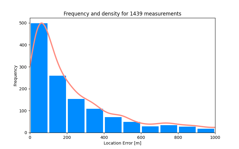
Processing 1439 measurements from sets 1+2+3+4+5+6+7+8: 100%
2021-11-18 13:11:03,549 Stop MPyC runtime -- elapsed time: 0:00:54.634274
Location Error [m]:
count 1439.000000
mean 702.527331
std 1875.874072
min 0.304723
25% 67.862993
50% 183.571693
75% 487.555568
max 17650.578739
dtype: float64
The error is limited to a few hundred meters, which can also be seen from the histogram and density plot:
Technically, our implementation of Schmidt’s method reuses function linear_solve() from the
demo ridgeregression.py
to compute the required least-squares approximation entirely over the integers. In the example run shown here
we use secure 335-bit integers for an accuracy of 3 decimal places (scale factor of 1000). Varying the accuracy
from 6 decimal places (using 470-bit integers) to 0 decimal places (using 200-bit integers) has little
impact on the results nor on the performance.
See multilateration.py for more information.
kmsurvival.py
This demo is about privacy-preserving Kaplan–Meier survival analysis. For an extensive explanation we refer to the Jupyter notebook KaplanMeierSurvivalExplained.ipynb.
A run for the aml.csv dataset gives the following numbers:
$ python kmsurvival.py --no-log -M3 -i2
Using secure fixed-point numbers: SecFxp64:32
Dataset: aml, with 3-party split, time 1 to 161 (stride 16) weeks
Chi2=3.396389, p=0.065339 for all events in the clear
Chi2=0.411455, p=0.521232 for own events in the clear
Chi2=2.685357, p=0.101275 for aggregated events in the clear
Chi2=3.396385, p=0.065339 for all events secure, exploiting aggregates
Chi2=3.396390, p=0.065339 for all 161 time moments secure
The demo makes essential use of secure fixed-point numbers to do the necessary computations for the
logrank tests that are used to see if there is a significant difference between two survival curves.
For the purpose of the demo, we partition the given dataset aml evenly between the 3 parties
running the demo in this example. This is accomplished by the following line of code, where df is
a pandas.DataFrame:
df = df[mpc.pid::m] # simple partition of dataset between m parties
In total, we perform the logrank test in five different ways, for varying trade-offs between efficiency and security.
The demo also supports plotting. For instance, as a somewhat “differentially private” view of the actual survival curves held in secret-shared form between the parties, we have the following aggregated view:
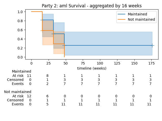
For a properly selected aggregation period, the information leakage on individual events may be acceptable, at the same time ensuring that the plot still gives a useful impression of the situation.
See kmsurvival.py for more information. Also see the vectorized version np_kmsurvival.py, using secure NumPy arrays for more efficient MPyC code.
cnnmnist.py
This demo shows a fully private Convolutional Neural Network (CNN) classifier at work for the MNIST dataset of handwritten digits.
Both the CNN parameters (neuron weights and bias for all layers) and the test images are kept secret throughout the entire multiparty computation.
A run of the demo looks as follows:
$ python cnnmnist.py -M3
2021-06-24 18:10:44,100 Start MPyC runtime v0.7.7
2021-06-24 18:10:44,616 All 3 parties connected.
2021-06-24 18:10:44,616 --------------- INPUT   -------------
Type = SecInt37, range = (2830, 2831)
Labels: [6]
[[0000000000000000000000000000]
 [0000000000000000000000000000]
 [0000000011110000000000000000]
 [0000000011110000000000000000]
 [0000000111110000000000000000]
 [0000000111100000000000000000]
 [0000000111100000000000000000]
 [0000000111100000000000000000]
 [0000000111100000000000000000]
 [0000001111100000111110000000]
 [0000001111101111111111100000]
 [0000001111111111111111110000]
 [0000001111111111111111111000]
 [0000001111111111111111111000]
 [0000001111111111000011111000]
 [0000000111111100000011111000]
 [0000000111111111000011111000]
 [0000000011111111111111111000]
 [0000000011111111111111111000]
 [0000000001111111111111111000]
 [0000000000111111111111111000]
 [0000000000000111111111100000]
 [0000000000000000000000000000]
 [0000000000000000000000000000]
 [0000000000000000000000000000]
 [0000000000000000000000000000]
 [0000000000000000000000000000]
 [0000000000000000000000000000]]
2021-06-24 18:10:44,709 --------------- LAYER 1 -------------
2021-06-24 18:10:44,725 - - - - - - - - conv2d  - - - - - - -
2021-06-24 18:10:45,662 - - - - - - - - maxpool - - - - - - -
2021-06-24 18:11:49,392 - - - - - - - - ReLU    - - - - - - -
2021-06-24 18:12:08,453 --------------- LAYER 2 -------------
2021-06-24 18:12:08,578 - - - - - - - - conv2d  - - - - - - -
2021-06-24 18:12:16,437 - - - - - - - - maxpool - - - - - - -
2021-06-24 18:12:48,028 - - - - - - - - ReLU    - - - - - - -
2021-06-24 18:12:56,762 --------------- LAYER 3 -------------
2021-06-24 18:13:03,621 - - - - - - - - fc      - - - - - - -
2021-06-24 18:13:04,621 - - - - - - - - ReLU    - - - - - - -
2021-06-24 18:13:10,355 --------------- LAYER 4 -------------
2021-06-24 18:13:10,621 - - - - - - - - fc      - - - - - - -
2021-06-24 18:13:10,621 --------------- OUTPUT  -------------
Image #2830 with label 6: 6 predicted.
[-3961968811, -11882041148, -13312379672, -13152456612, -2770332627, 4413001565, 26611143242, -14166673783, -1258705244, -11310948875]
2021-06-24 18:13:10,683 Stop MPyC runtime -- elapsed time: 0:02:26.583087
The lines printed by mpc.barrier() have been removed for brevity.
The barriers are inserted to speed up the overall computation: without any barriers the MPyC program
will first build the “circuit” for the complete neural network, before evaluating any “gate” of this
circuit. Placement of the barriers ensures that the “circuit” is divided into more manageable
parts, such that the parties have sufficiently many “gates” to work on in parallel.
See cnnmnist.py for more information.
Also see the vectorized version np_cnnmnist.py, using secure NumPy arrays for more compact and more efficient MPyC code.
bnnmnist.py
This demo presents an alternative fully private MNIST classifier, namely a Binarized Neural Network (Multilayer Perceptron) classifier.
The layers of the network are fully connected to each other, and all weights in the network as well as the values of the activation functions have been “binarized”, that is, mapped to 1 or -1. Also, we use a special type of secure comparison protocol to speed up the activation functions.
A run for a batch of 8 digits looks as follows:
$ python bnnmnist.py -M3 -o2830 -b8
2021-06-24 18:36:19,458 Start MPyC runtime v0.7.7
2021-06-24 18:36:19,974 All 3 parties connected.
2021-06-24 18:36:19,974 --------------- INPUT   -------------
Type = SecInt14(9409569905028393239), range = (2830, 2838)
Labels: [6, 6, 5, 7, 8, 4, 4, 7]
2021-06-24 18:36:20,052 --------------- LAYER 1 -------------
2021-06-24 18:36:20,052 - - - - - - - - fc      - - - - - - -
2021-06-24 18:36:20,583 - - - - - - - - bsgn    - - - - - - -
2021-06-24 18:37:10,455 --------------- LAYER 2 -------------
2021-06-24 18:37:10,455 - - - - - - - - fc      - - - - - - -
2021-06-24 18:38:01,876 - - - - - - - - bsgn    - - - - - - -
2021-06-24 18:38:07,720 --------------- LAYER 3 -------------
2021-06-24 18:38:07,720 - - - - - - - - fc      - - - - - - -
2021-06-24 18:38:55,669 - - - - - - - - bsgn    - - - - - - -
2021-06-24 18:39:01,685 --------------- LAYER 4 -------------
2021-06-24 18:39:01,685 - - - - - - - - fc      - - - - - - -
2021-06-24 18:39:01,841 --------------- OUTPUT  -------------
Image #2830 with label 6: 6 predicted.
[-723, -620, -613, -552, -718, -687, 1042, -901, -567, -570]
Image #2831 with label 6: 6 predicted.
[-517, -608, -437, -368, -538, -249, 564, -1273, -683, -478]
Image #2832 with label 5: 5 predicted.
[-652, -581, -464, -675, -443, 840, -463, -340, -532, -559]
Image #2833 with label 7: 7 predicted.
[-566, -603, -590, -487, -497, -1312, -1707, 786, -486, -701]
Image #2834 with label 8: 8 predicted.
[-469, -724, -569, -590, -592, -621, -734, -543, 957, -514]
Image #2835 with label 4: 4 predicted.
[-455, -500, -607, -524, 940, -407, -540, -523, -441, -704]
Image #2836 with label 4: 4 predicted.
[-599, -260, -385, -460, 146, -559, -934, -387, -749, -648]
Image #2837 with label 7: 7 predicted.
[-532, -603, -588, -397, -357, -1764, -1697, 770, -396, -511]
2021-06-24 18:39:02,044 Stop MPyC runtime -- elapsed time: 0:02:42.585459
Note that SecInt14(9409569905028393239) is used as secure type.
These are 14-bit secure integers, where \(p=9409569905028393239\) is the prime
that we have set for the underlying finite field to be used for Shamir secret sharing.
The prime \(p\) is selected to get a fast protocol for secure comparisons,
exploiting properties of the Legendre symbol of integers modulo \(p\).
See bnnmnist.py for more information.
Also see the vectorized version np_bnnmnist.py, using secure NumPy arrays for more compact and more efficient MPyC code.
[np-]run-all.{bat,sh}
All the demos from helloworld.py up to dsa.py can be run in one go using
run-all.bat or
run-all.sh.
These demos have no dependencies other than MPyC itself.
You can also provide parameters like -M 3 to run all demos with three parties.
Similarly, the demos sha3.py and pseudoinverse.py as well as all available “vectorized” versions
of the demos (np_id3gini.py, np_cnnmnist.py, and so on) can be run using
np-run-all.bat or
np-run-all.sh.
These demos use MPyC’s secure arrays and all require NumPy.